
For obvious reasons, we model cloud environments as part of the enterprise architecture universe. SAMU’s API and the data synchronization module enable our clients to integrate SAMU to basically anything and exchange data. In this demo we used the sync module to create a data stream from the ever-changing Amazon Web Services and visualize it.
You see the video below, but let me sum up how I did it:
1. Setup the trial AWS account and an empty SAMU application
I created a test AWS account with few free-tier services (EC2, RDS, VPCs, etc). Beyond the basic attributes of the services, I also wanted to link them to higher architecture components, such as business applications they are used for. Therefore, I made a template for provisioning new AWS resources with two tags: App tag includes the name of the application the server / RDS is used for and a Purpose tag, which refers to the type of the environment, eg. Production / Test / Development / etc. You’ll see soon, how we are using these…
I also installed an empty SAMU repository, where we’ll load the data to.
2. Query AWS info through CLI
You can query a wealth of environmental information through the AWS Command Line Interface, which I used for the purpose of the demo. With few shell scripts I generated CSV files that contained basic information about the EC2 instances, the RDS I’m using and other components, such as the availability zones, virtual private clouds and so on.
Note that you don’t need to create CSVs, but can load them into temp SQL tables, for example.
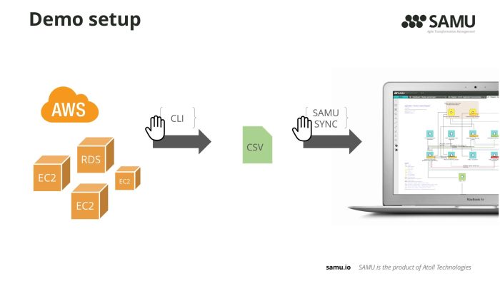
3. Define sync jobs in SAMU Sync module to load the CSV files into SAMU
SAMU natively offers an Excel importing wizard for users to perform easy data bulk loads. Instead of using that, I opted for the SAMU Sync module in order to define sync jobs which can be executed automatically. I will start the first job manually (so you would see it working) and all the subsequent jobs run automatically.
4. Log in SAMU and visualize the AWS environment
Once the data is in SAMU, the tool can visualize any segment of the architecture graph. Since dependencies and relationships among various components come across the integration, you can browse and drill down into any area.
For instance, we load EC2 instances as objects in SAMU and we also load availability zones and regions as objects too. We relate the relevant objects, eg EC2 XYZ operates in Region us-east-2. You can click the Region us-east-2 and drill down to visualize all EC2 instances as well as RDS instances related to it.
Location view in SAMU generated for a selected region (us-east-2). It displays the services (EC2 and RDS) within the availability zones. It also shows the business applications the services are used for (linked to the application’s various environments, such as production / test / development / etc). You can open the data sheet of any components in SAMU and see the attributes we pulled over from AWS.
As said, I added two tags for each EC2 and RDS: App and Purpose. During the data sync I create (or update if existing) Application objects corresponding to the value of the App tag. In our best practice meta-model we have an intermediary component between Applications and Virtual Servers, which we call Application Environment. Application Environments represent the running instances of the logical applications. For example if you look at SAMU Application, you might have a SAMU Production Application Environment, but also a SAMU Test or SAMU Sandbox environments – all of them running on perhaps different set of Virtual Servers. In the demo, I also create Application Environments automatically based on these two tags.

Nikoletta Csonka leads SEO and content strategy at Atoll Technologies, aligning digital visibility with business goals. She focuses on search-driven content development, thought leadership, and employer branding communication to strengthen Atoll’s market positioning.
With a data-informed and audience-centric approach, Nikoletta ensures that content not only ranks well but also builds credibility and long-term brand value.